1. Introduction
Energy is a major challenge in most developing countries. Nearly 567 million people in Sub-Saharan Africa do not have access to electricity
. Zimbabwe is within the Sub-Saharan regions of Africa and is not immune to such prevailing energy challenges
| [2] | T. C. Maramura, E. T. Maziriri, T. Chuchu, D. Mago, and R. Mazivisa, ‘RENEWABLE ENERGY ACCESS CHALLENGE AT HOUSEHOLD LEVEL FOR THE POOR IN RURAL ZIMBABWE: IS BIOGAS ENERGY A REMEDY?’, IJEEP, vol. 10, no. 4, pp. 282-292, May 2020, https://doi.org/10.32479/ijeep.8801. |
[2]
. Most countries are still relying on fossil fuels for power generation which are finite and less environmentally friendly. Some countries are moving away from the use of fossil fuels to infinite sources of energy such as hydro, solar and wind. Zimbabwe just like other developing countries is not an exception. The country has reported increase in the power demand and electricity shortages evidenced by frequent power cuts
| [3] | A. B. Maqhuzu, K. Yoshikawa, and F. Takahashi, ‘The effect of coal alternative fuel from municipal solid wastes employing hydrothermal carbonization on atmospheric pollutant emissions in Zimbabwe’, Science of The Total Environment, vol. 668, pp. 743-759, Jun. 2019, https://doi.org/10.1016/j.scitotenv.2019.03.050 . |
| [4] | K. Nyavaya, ‘Clean energy: The untapped solution to Zimbabwe’s power crisis’, Mar. 02, 2023. [Online]. Available: https://energytransition.org/2023/03/clean-energy-the-untapped-solution-to-zimbabwes-power-crisis/ |
| [5] | S. Ziuku, L. Seyitini, B. Mapurisa, D. Chikodzi, and K. Van Kuijk, ‘Potential of Concentrated Solar Power (CSP) in Zimbabwe’, Energy for Sustainable Development, vol. 23, pp. 220-227, Dec. 2014, https://doi.org/10.1016/j.esd.2014.07.006 |
[3-5]
. Reduction in water levels for hydroelectricity in Kariba dam
| [6] | R. Runganga and S. Mishi, ‘Modelling Electric Power Consumption, Energy Consumption and Economic Growth in Zimbabwe: Cointegration and Causality Analysis’, American Journal of Economics, 2020. |
[6]
, increase in energy demand from the growing population, mining and agriculture sector has attributed energy shortages in the nation
. To meet this growing demand of energy in Zimbabwe there is need for significant expansion in energy generation in a multidimensional way through the incorporation of sustainable energies such as solar, wind, hydrogen etc. Solar energy from the sun is the most copious natural resource, free, and is found everywhere. Solar energy can be utilized to provide triple panacea for the country which are to reduce energy deficit, diminish greenhouse gas emission from thermal energy sources and minimize forest degradation from cutting down of trees for firewood and charcoal. Sustainable energies to be specific solar energy, can be a game changer for many developing countries such as Zimbabwe because of its abundance, cost competitiveness and reliability. Zimbabwe is driving towards sustainable economic development through affordable, reliable and modern energies following the United Nations Sustainable Development Goals (UN-SDG) number 7. Through its Vision 2030 the government of Zimbabwe has committed to reduce reliance on fossil fuels in accordance to the UN-SDG number 13 (Climate action). It is therefore imperative to consider solar radiation as a source of energy in order to tackle the energy shortages in the country. The efficiency of solar systems depends on the amount of solar radiation received therefore it is of paramount importance to model and map received ground solar radiation, because it changes with time, which is the premise of this research. It therefore becomes this research’s thrust to determine how ground solar radiation varies, where it varies and when it varies and the processes behind this variation. Geospatial techniques embedded in python programming also coupled with solar radiation equations and radiation models were used to determine the availability of solar energy by predicting variations in clear sky solar radiation. The quantity of solar energy varies with geographical location, sun position, time, terrain (slope and aspect), atmospheric constituencies and thickness etc. At any given time, solar radiation varies in geographic space principally from changes in solar angles at any given set of 3D coordinates (latitude, longitude and elevation). Variations in these temporal and spatial factors are vital in determining the total solar radiation received per hour, day, month, and year. Algorithms for timely solar radiation quantification have been developed in many countries which is an urgent crevice in Zimbabwe that needs to be filled by adopting geospatial techniques, programming and radiation equations. An alternative way to obtain solar radiation data is through numerical models
| [8] | M. A. A. Al-Dabbas, ‘The Analysis of the Characteristics of the Solar Radiation Climate of the Daily Global Radiation And Diffuse Radiation in Amman, Jordan’, vol. 5, no. 2, 2010. |
[8]
. Clear sky radiation models measures the amount of solar radiation received per area when there are no clouds interference and, some incorporate the effects of geo-variables such as latitude, longitude, elevation, surface albedo, and Earth-Sun distance
| [9] | X. Sun, J. M. Bright, C. A. Gueymard, B. Acord, P. Wang, and N. A. Engerer, ‘Worldwide performance assessment of 75 global clear-sky irradiance models using Principal Component Analysis’, Renewable and Sustainable Energy Reviews, vol. 111, pp. 550-570, Sep. 2019, https://doi.org/10.1016/j.rser.2019.04.006 |
[9]
. Solar models dates back to 1940’s and they differ in precision, complexity and required input data
| [10] | A. J. Gutiérrez-Trashorras, E. Villicaña-Ortiz, E. Álvarez-Álvarez, J. M. González-Caballín, J. Xiberta-Bernat, and M. J. Suarez-López, ‘Attenuation processes of solar radiation. Application to the quantification of direct and diffuse solar irradiances on horizontal surfaces in Mexico by means of an overall atmospheric transmittance’, Renewable and Sustainable Energy Reviews, vol. 81, pp. 93-106, Jan. 2018, https://doi.org/10.1016/j.rser.2017.07.042 |
[10]
.
| [11] | I. Reda and A. Andreas, ‘Solar Position Algorithm for Solar Radiation Applications (Revised)’, NREL/TP-560-34302, 15003974, Jan. 2008. https://doi.org/10.2172/15003974 . |
[11]
Used solar algorithms for calculating sun position, solar geometry angles such solar zenith, azimuth angles and other parameters related with an uncertainty of ±0.0003. Solar geometry angles such as solar azimuth, solar elevation, and solar zenith has been used for developing sun tracking algorithms
| [12] | A. A. Rizvi, K. Addoweesh, A. El-Leathy, and H. Al-Ansary, ‘Sun position algorithm for sun tracking applications’, in IECON 2014 - 40th Annual Conference of the IEEE Industrial Electronics Society, Dallas, TX, USA: IEEE, Oct. 2014, pp. 5595-5598. https://doi.org/10.1109/IECON.2014.7049356 |
[12]
. The amount of solar radiation received by the surface depends on stochastic and deterministic factors which includes day of the year, geographic latitude, time of the day, solar geometric angles
| [13] | S. G. Obukhov, I. A. Plotnikov, and V. G. Masolov, ‘Mathematical model of solar radiation based on climatological data from NASA SSE’, IOP Conf. Ser.: Mater. Sci. Eng., vol. 363, p. 012021, May 2018, https://doi.org/10.1088/1757-899X/363/1/012021 |
[13]
. Clear sky models are used to determine the quantity of solar irradiance received by the earth’s surface under cloudless atmospheric conditions
| [14] | B. Mabasa, M. D. Lysko, H. Tazvinga, N. Zwane, and S. J. Moloi, ‘The Performance Assessment of Six Global Horizontal Irradiance Clear Sky Models in Six Climatological Regions in South Africa’, Energies, vol. 14, no. 9, p. 2583, Apr. 2021, https://doi.org/10.3390/en14092583. |
[14]
. The estimated solar radiation arising from clear sky models is given as either one or a combination of the irradiance components known as direct, diffuse and global
| [15] | L. Javu, H. Winkler, and K. Roro, ‘VALIDATING CLEAR-SKY IRRADIANCE MODELS IN FIVE SOUTH AFRICAN LOCATIONS’. |
[15]
. For a given location on the surface of the earth the hotel clear sky model can estimate the clear sky beam solar radiation (Gcb), taking into account the solar zenith angle, altitude and standard atmosphere for a four different climatic region using a set of equations
| [16] | C. Lingamgunta and T. Nejat Veziroglu, ‘A universal relationship for estimating daily clear sky insolation’, Energy Conversion and Management, vol. 45, no. 15-16, pp. 2313-2333, Sep. 2004, https://doi.org/10.1016/j.enconman.2003.11.019 |
[16]
. Equations for estimating clear sky diffuse solar radiation (Gcd) were laid out by
| [17] | B. Y. H. Liu and R. C. Jordan, ‘The interrelationship and characteristic distribution of direct, diffuse and total solar radiation’, Solar Energy, vol. 4, no. 3, pp. 1-19, Jul. 1960, https://doi.org/10.1016/0038-092X(60)90062-1 . |
[17]
. Total solar radiation combines the beam radiation, diffuse radiation and ground reflected radiation as explained by
| [16] | C. Lingamgunta and T. Nejat Veziroglu, ‘A universal relationship for estimating daily clear sky insolation’, Energy Conversion and Management, vol. 45, no. 15-16, pp. 2313-2333, Sep. 2004, https://doi.org/10.1016/j.enconman.2003.11.019 |
| [17] | B. Y. H. Liu and R. C. Jordan, ‘The interrelationship and characteristic distribution of direct, diffuse and total solar radiation’, Solar Energy, vol. 4, no. 3, pp. 1-19, Jul. 1960, https://doi.org/10.1016/0038-092X(60)90062-1 . |
| [18] | J. A. Duffie and W. A. Beckman, Solar Engineering of Thermal Processes, 4th ed. Hoboken, New Jersey: John Wiley & Sons, Inc., 2013. |
[16-18]
.
| [19] | A. A. El-Sebaii, F. S. Al-Hazmi, A. A. Al-Ghamdi, and S. J. Yaghmour, ‘Global, direct and diffuse solar radiation on horizontal and tilted surfaces in Jeddah, Saudi Arabia’, Applied Energy, vol. 87, no. 2, pp. 568-576, Feb. 2010, https://doi.org/10.1016/j.apenergy.2009.06.032 |
[19]
suggested models for calculating total incident radiation on horizontal and tilted surfaces and found a fair agreement between radiation models and ground observations. Ground radiation data and data derived from the clear sky model were used by
| [20] | N. Nijegorodov, ‘Improved ashrae model to predict hourly and daily solar radiation components in Botswana, Namibia, and Zimbabwe’, Renewable Energy, vol. 9, no. 1-4, pp. 1270-1273, Sep. 1996, https://doi.org/10.1016/0960-1481(96)88508-9 |
[20]
to come up with improved empirical coefficient values for Botswana, Namibia and Zimbabwe. Also in Zimbabwe solar radiation location-based coefficients have been developed by
| [21] | C. Iradukunda and K. Chiteka, ‘Angstrom-Prescott Type Models for Predicting Solar Irradiation for Different Locations in Zimbabwe’, sv-jme, vol. 69, no. 1-2, pp. 32-48, Feb. 2023, https://doi.org/10.5545/sv-jme.2022.331 |
[21]
using linear correlation between solar radiation and sunshine duration. This work therefore presents a system for timely solar radiation estimation and an annual average radiation map which is a product of different weighted radiation datasets. The study also assessed and identified regions in Zimbabwe that are suitable for medium to large scale Photovoltaic (PV) solar plants installations.
2. Materials and Methods
2.1. Study Area
Zimbabwe is a landlocked Southern African country which boarders South Africa to the south, Botswana to the west, Zambia to the north and Mozambique to the east
| [21] | C. Iradukunda and K. Chiteka, ‘Angstrom-Prescott Type Models for Predicting Solar Irradiation for Different Locations in Zimbabwe’, sv-jme, vol. 69, no. 1-2, pp. 32-48, Feb. 2023, https://doi.org/10.5545/sv-jme.2022.331 |
[21]
as shown in
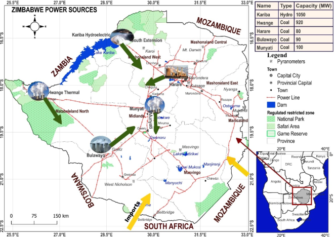
Figure 1. The country is located within the subtropical climate and receives plentiful sunshine. World regions such as Zimbabwe are gifted with plentiful amount of annual solar radiation. The study area lies within latitude 15.6S
o to 22.4
oS, longitude 25.3
o E to 33.1
oE. It encompasses an area of 390,757
. Altitude ranges between 300m and 2500m above mean sea level (m.s.l). Higher altitudes (>1000m) receive higher amounts of precipitation and experience cooler temperatures compared to regions of lower altitude. Zimbabwe is divided into five agro-ecological zones which are classified by rainfall and weather patterns with the regions receiving highest rainfall being 1 and 2A, region 2B and 3 receive average rainfall and regions 4 and 5 receive the lowest rainfall
. The average temperature per year is 15°C in winter to 26°C in summer. Zimbabwe has three recognizable seasons which are summer season which stretches from November to March, winter season which spans from April to July and the spring or hot and dry season which stretches from August to mid-November
| [22] | I. Gwitira et al., ‘GIS-based stratification of malaria risk zones for Zimbabwe’, Geocarto International, vol. 34, no. 11, pp. 1163-1176, Sep. 2019, https://doi.org/10.1080/10106049.2018.1478889 |
| [23] | M. Manjowe, T. Mushore, E. Matandirotya, and E. Mashonjowa, ‘Characterisation of wet and dry summer seasons and their spatial modes of variability over Zimbabwe’, S. Afr. J. Sci., vol. 116, no. 7/8, Jul. 2020, https://doi.org/10.17159/sajs.2020/6517 |
| [24] | L. Unganai, ‘Historic and future climatic change in Zimbabwe’, Clim. Res., vol. 6, pp. 137-145, 1996, https://doi.org/10.3354/cr006137 |
[22-24]
. Zimbabwe’s population is about 15.18 million where 48% are male and 52% are female (ZIMSTAT, 2022). The country’s major sources of energy are thermal from coal and hydroelectricity. The major coal power plants are Hwange, Bulawayo, Harare and Munyati. Hydroelectricity is generated from the Kariba dam and other mini hydropower stations.
Figure 1. Study area map.
2.2. Data Source
Data for the study was acquired from various sources as shown in
Table 1.
Table 1. Data Source.
Data | Source | Use |
Monthly average radiation measured by pyranometers | Meteorological Services Department (MSD) of Zimbabwe | System calibration and validation |
SRTM DEM | USGS Earth Explorer | Elevation, Slope, Aspect |
Landsat 5 (path 168 to 173, row 71 to 75) | USGS Earth Explorer | Surface Albedo |
Average Annual Temperature | Global Solar Atlas | Site Suitability Analysis |
Landcover | Copernicus Global Land Service | Site Suitability Analysis |
River, Dams, Roads, Rail, Powerlines, Protected areas | Open Street Map (OSM) | Site Suitability Analysis |
Province and District | Humanitarian data exchange | Boundary |
2.3. Data Preparation
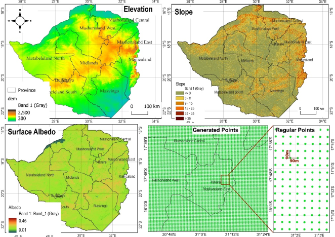
Figure 2. Input data map; Elevation (a), Slope (b), Surface Albedo(c), Regular Points (d).
The initial process for this study was data gathering and preparation. The system for radiation depends on other geospatial datasets such as Digital Elevation Models (DEM), slope and surface albedo. These datasets were input variables in solar radiation equations as they have significant influence on the amount of received radiation. For a continuous surface of elevation, Shuttle Radar Topographic Models (SRTM) - DEM for the whole of Zimbabwe was used. Elevation shown in
Figure 2(a) was a crucial parameter in hotel clear sky radiation model as it correlates strong with surface radiation. Slope is an elevation derivative which show irregularities in terrain. Slope is also known as the degree of change in surface elevation
Figure 2(b). Slope is key in radiation calculation as it shows the tilt angle of the surface from the horizontal normal. The spatial variation in slope tends to influence variation in ground received radiation and the total radiation received per day. Slope also affect the sunrise and the sunset hour angles thereby affecting the amount of sunshine hours. Surface albedo is the reflectivity of the surface which is principally determined by the landuse and landcover of the surface. Surface albedo has an influence on ground reflected radiation. The method by
| [25] | S. Liang, ‘Narrowband to broadband conversions of land surface albedo I Algorithms’, Remote Sensing of Environment, 2000. |
| [26] | R. B. Smith, ‘The heat budget of the earth’s surface deduced from space’, 2010. |
[25, 26]
was used to calculate surface albedo for the whole of Zimbabwe using Landsat 5 satellite imagery. Since the in-situ radiation data for validation starts from 2006, therefore Landsat 5 images were downloaded for 2006. To convert Digital Number (
DN) values to reflectance values pre-processing was performed in QGIS using the Semi-Automatic Classification Plugin.
(1)
Where ρi corresponds to the surface reflectance of the Landsat 5 ith band.
2.4. Generating Regular Points
For efficiency of the system there was need to balance execution time and file sizes of input data. Large file sizes for DEM, slope and albedo about 2GB for each raster datasets were slowing the processing time for the system. To balance this trade-off regularly spaced points were generated in QGIS. These points were 90m apart in both x and y directions as shown in
Figure 2(d). Elevation, slope and albedo were resampled from 30m resolution to 90m. Point Sampling tool, a QGIS plugin was used to get the corresponding pixel values for elevation, slope and albedo for each generated point. The point data was exported as a csv file which contains latitude, longitude extracted elevation, slope and albedo values of each point. This csv file is less heavy when opened in python as compared to opening 3 raster files at once. This increased the system efficiency.
2.5. System Design
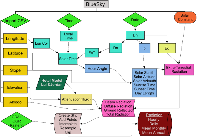
Figure 3. System Flowchart.
System design and automation of ground received solar radiation was done using python programming. The initial step was to install all the required python packages/modules for system development. Geospatial Data Abstraction Library (GDAL) is the bedrock of the developed system as it handles all the spatial data and spatial analysis. Numeric Python (numpy) and math packages are strong in handling mathematical computations especial radiation models and equations. Rasterio is another python package which was used interchangeably with GDAL in handling of raster data. Received solar radiation is time dependant therefore the datetime, calendar and time modules were used. Pandas was used to open and handle the csv files. For plotting and displaying of images and graphs, matplotlib package was used. The system required a Graphic User Interface (GUI) for displaying results and execution of commands therefore
Tk interface also known as tkinter module was used to create buttons, entry boxes and radio buttons. A system for automated ground solar radiation prediction nicknamed BlueSky (since it estimates clear sky solar radiation) was developed using a series of interlinked radiation equations as shown in
Figure 3 to determine solar radiation per site, sun position and path. Using the solar geometry equations, the position of the sun can be tracked at any time of the day. Solar angles equations from
| [18] | J. A. Duffie and W. A. Beckman, Solar Engineering of Thermal Processes, 4th ed. Hoboken, New Jersey: John Wiley & Sons, Inc., 2013. |
[18]
were used. The following equations were handled using math and numpy modules.
2.5.1. Declination Angle (𝛿)
This is the angle between the equatorial plane and the Sun's direction and ranges between -23.45
o to 23.45. It is also known as the tilt angle of the earth and is responsible for the daily changes in received solar radiation. This angular position of the sun is dependent on day number (dn) of the year and the location of the place relative to the equator. It is expressed as
| [18] | J. A. Duffie and W. A. Beckman, Solar Engineering of Thermal Processes, 4th ed. Hoboken, New Jersey: John Wiley & Sons, Inc., 2013. |
[18]
.
(2)
2.5.2. Eccentricity Correction Factor (Eo)
Due to the earth’s elliptical orbit around the sun, the actual extra-terrestrial (outside earth atmosphere) solar radiation varies from the solar constant. Eccentricity correction factor takes care of the variations in solar radiation as a result of changes in sun-earth distance, as the earth revolves around its orbit and can be expressed by the following
| [18] | J. A. Duffie and W. A. Beckman, Solar Engineering of Thermal Processes, 4th ed. Hoboken, New Jersey: John Wiley & Sons, Inc., 2013. |
[18]
.
2.5.3. Equation of Time (EoT)
It gives the difference between local solar time and the clock time. It sets the time from the standard clock to uniform throughout all the places within the same time zones
(4)
Where:
(i). Time Correction (Tc)
Time correction was performed because not all places within a given time zone are located at the Local standard time meridian (LSTM). Time correction uses the longitude of the site of interest, LSTM, and Equation of time. It takes 4 minutes for the sun to pass 1o of Longitude.
(6)
(ii). Solar Time
Local solar time (LST) equations set every place within the same time zone to be in tandem with the time at LSTM. It makes use of the local clock time and the time correction factor.
2.5.4. Hour Angle (ω)
It’s a known fact the earth takes a day (24hours) to make a 360
o rotation
| [18] | J. A. Duffie and W. A. Beckman, Solar Engineering of Thermal Processes, 4th ed. Hoboken, New Jersey: John Wiley & Sons, Inc., 2013. |
[18]
. Dividing 360
o by 24hrs it means 1hour is equivalent to 15
o of longitude
. Therefore, hour angle is the representation of hours after 12 midnight in degrees.
(i). Sunrise and Sunset Time
Most photovoltaic solar panels efficiently harness meaningful economic amounts of radiation post-sunrise and pre-sunset. The BlueSky was designed to estimate solar radiation between sunrise and sunset time. Sunrise time is calculated from sunrise hour angle which is expressed by the following formula.
(9)
Where the latitude, β is inclination angle of the surface in this research it is represented by slope and δ is the declination angle.
(ii). Day Length (DL)
Day length can be a proxy for the number of sunshine hours. The number of hours the surface receives sunlight correlates with amount of radiation received.
(12)
2.5.5. Solar Altitude Angle (α) and Solar Zenith Angle (θ)
To estimate the amount of solar radiation reaching the earth’s surface it is extremely crucial to solve the trigonometric relationships between the position of the sun in the sky and the surface coordinates. These trigonometric relationships are used in solar tracking. Solar altitude is the angle of the sun relative to the surface horizon and solar zenith is angle between the nadir and the line joining the sun and the site of interest. Solar zenith is the conjugate angle of solar altitude above the horizon. The angles were calculated in degrees and they complement each other (θ + α = 90°). These angles depend on latitude, time of the day, declination angle and slope. Solar zenith angle is 90° at sunrise and sunset at that time solar altitude is 0°. At 12 noon solar zenith is assumed to be 0° and solar altitude is 90°. When zenith angle is closer to 0 solar rays travel less distance in the atmosphere to the ground which implies little interaction between incoming radiation and atmospheric constituencies resulting in high solar radiation during mid-day hours.
(13)
2.5.6. Solar Constant (Gsc)
This is the energy from the sun received on a unit area per unit of time. It is measured per unit of area which is perpendicular to the extra-terrestrial radiation at mean earth sun distance (1.496* 10
11m). This research used the value of 1367W/m
2 which was adopted by World Radiation Centre (WRC) as solar constant
| [18] | J. A. Duffie and W. A. Beckman, Solar Engineering of Thermal Processes, 4th ed. Hoboken, New Jersey: John Wiley & Sons, Inc., 2013. |
[18]
.
2.5.7. Hotel Clear Sky Model
The estimation of solar radiation received on a clear day was computed using Hotel clear sky model. The model calculate direct and diffuse solar radiation on a clear day and atmospheric attenuation are taken care by the transmittance coefficient (τb) and dispersion coefficient (τd)
| [10] | A. J. Gutiérrez-Trashorras, E. Villicaña-Ortiz, E. Álvarez-Álvarez, J. M. González-Caballín, J. Xiberta-Bernat, and M. J. Suarez-López, ‘Attenuation processes of solar radiation. Application to the quantification of direct and diffuse solar irradiances on horizontal surfaces in Mexico by means of an overall atmospheric transmittance’, Renewable and Sustainable Energy Reviews, vol. 81, pp. 93-106, Jan. 2018, https://doi.org/10.1016/j.rser.2017.07.042 |
| [13] | S. G. Obukhov, I. A. Plotnikov, and V. G. Masolov, ‘Mathematical model of solar radiation based on climatological data from NASA SSE’, IOP Conf. Ser.: Mater. Sci. Eng., vol. 363, p. 012021, May 2018, https://doi.org/10.1088/1757-899X/363/1/012021 |
| [17] | B. Y. H. Liu and R. C. Jordan, ‘The interrelationship and characteristic distribution of direct, diffuse and total solar radiation’, Solar Energy, vol. 4, no. 3, pp. 1-19, Jul. 1960, https://doi.org/10.1016/0038-092X(60)90062-1 . |
| [18] | J. A. Duffie and W. A. Beckman, Solar Engineering of Thermal Processes, 4th ed. Hoboken, New Jersey: John Wiley & Sons, Inc., 2013. |
[10, 13, 17, 18]
. The model makes use of the zenith angle, elevation and climate type. The hotel model made use of Equations 14 - 18 and parameters in
Table 2.
(14)
(15)
(16)
Where A is elevation in kilometres for areas with altitude less than 2.5km. Correlation factors (
allow for changes in climate types and are shown in
Table 2. Transmittance
and dispersion coefficient
are calculated as follows.
(18)
Table 2. Correlation factors for climatic types.
Climate Type | | | |
Tropical | 0.95 | 0.98 | 1.02 |
Midlatitude summer | 0.97 | 0.99 | 1.02 |
Midlatitude winter | 1.03 | 1.01 | 1.00 |
Subarctic summer | 0.99 | 0.99 | 1.01 |
(Hotel, 1976) correlation factors as cited by
| [18] | J. A. Duffie and W. A. Beckman, Solar Engineering of Thermal Processes, 4th ed. Hoboken, New Jersey: John Wiley & Sons, Inc., 2013. |
[18]
2.5.8. Extra-terrestrial Radiation
Hourly radiation outside of the earth’s atmosphere is product of solar constant (, eccentricity correction factor () and zenith angles at begin and end of hour.
(19)
Where and are hour angles at the begin and end of the hour.
(i). Beam Radiation
It is also known as direct solar radiation. It is the part of solar radiation, which travels unimpeded through space and the atmosphere to the surface. Hourly direct radiation was calculated as follows.
(ii). Diffuse Radiation
Received solar radiation after its direction has been altered by atmospheric scattering.
| [17] | B. Y. H. Liu and R. C. Jordan, ‘The interrelationship and characteristic distribution of direct, diffuse and total solar radiation’, Solar Energy, vol. 4, no. 3, pp. 1-19, Jul. 1960, https://doi.org/10.1016/0038-092X(60)90062-1 . |
[17]
Proposed the following formula for calculating diffuse radiation as:
(iii). Ground Reflected Radiation
The amount of radiation reflected by the surface is a function of ground albedo, caused by reflectance from the surrounding environments can be expressed as:
Where is ground albedo and is slope.
(iv). Global Horizontal Radiation
This is the total amount of radiation received on a surface expressed as:
Equations 2 - 23 were handled by numpy and math module. The system reads the csv file created in
Figure 2(d). Using the Pandas module, the csv was converted into an array. The system read latitude and longitude from the created numpy array using OpenGIS Simple Features Reference Implemetation (OGR) which is a vector library that comes with Geospatial Abstraction Library (GDAL). OGR creates a point shapefile and add the four attributes which are beam, diffuse, ground reflected and total hourly radiation. The system loops through all the points in the csv and calculated Equ.
2 - 23 for each point. Latitude, longitude, diffuse, beam, ground reflected and total are added to the created shapefile for each point. When the system loops through all the points in the csv, the shapefile were populated with radiation values for each point. GDAL was used to convert the created point shapefile into a raster file. Inverse distance weighting (IDW) was used to interpolate points with a power of 2, geotif format, minimum number of points of 4, and maximum number of points of 12. GDAL Warp was used to resample the created raster file to 90m spatial resolution using the nearest neighbour. In order for our radiation data to cover only Zimbabwe, clipping was applied on the resampled raster dataset.
2.5.9. Daily and Monthly Radiation
The BlueSky system calculates hourly radiation for hours within sunrise and sunset time. Daily radiation is the sum of hourly radiation within sunrise and sunset hours. Rasterio module was used to sum all hourly radiation datasets. Average amount of radiation received per month is the sum of all daily radiation divided by the number of days in that month.
2.6. Site Suitability Analysis
Suitable sites for solar power plants installation were determined using GIS and Multicriteria Decision Making process
| [5] | S. Ziuku, L. Seyitini, B. Mapurisa, D. Chikodzi, and K. Van Kuijk, ‘Potential of Concentrated Solar Power (CSP) in Zimbabwe’, Energy for Sustainable Development, vol. 23, pp. 220-227, Dec. 2014, https://doi.org/10.1016/j.esd.2014.07.006 |
| [27] | A. B. Jemaa, S. Rafa, N. Essounbouli, A. Hamzaoui, F. Hnaien, and F. Yalaoui, ‘Estimation of Global Solar Radiation Using Three Simple Methods’, Energy Procedia, vol. 42, pp. 406-415, 2013, https://doi.org/10.1016/j.egypro.2013.11.041 |
| [28] | I. I. Opeyemi, A. S. Abayomi, and G. Suara, ‘Site Suitability Assessment for Solar Photovoltaic Power Plant in FCT-Abuja, Nigeria: A Geographic Information System (GIS) and Analytical Hierarchy Process (AHP) Approach’, 2022. |
[5, 27, 28]
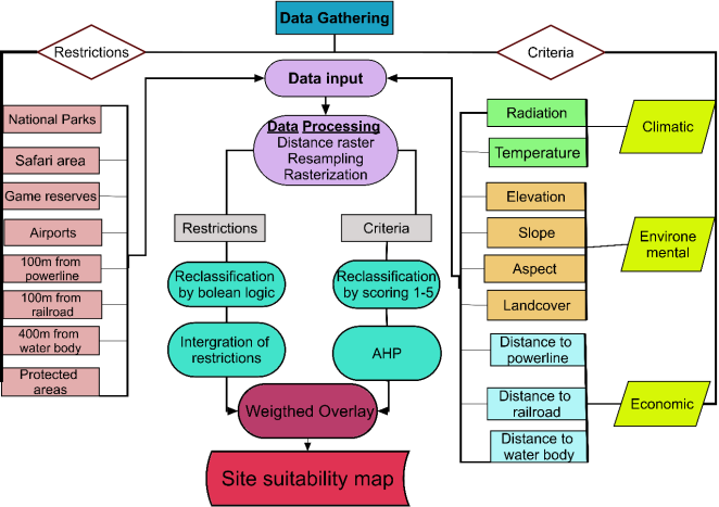
. Weighted overlay analysis was perform using nine factors which are annual average radiation, annual average temperature, elevation, slope, aspect, landcover, proximity to road, proximity to railroad and proximity to surface water bodies. The following framework was implemented in solar farm site suitable analysis.
2.7. Site Suitability Framework
The site suitability framework adopted is shown in
Figure 4.
Figure 4. Site suitability flowchart.
2.8. Data and Statistical Analysis
In-situ radiation data across 13 weather stations from 2006 to 2015 were obtained from Meteorological Services Department (MSD) of Zimbabwe. Data were divided into training and testing data. Training data were used to test the performance of monthly radiation whilst test data were used to evaluate the performance of annual average radiation. After developing the system, the next phase was performance assessment of the BlueSky system results against In-situ data. Data from the BlueSky system was tested for accuracy. Statistical metrics for relationships and dispersion were used to assess the performance of the system results together with other radiation datasets. SPSS, Microsoft excel and R Statistics were used for this analysis. Firstly, data were tested for normality using descriptive statistics and test statistics in SPSS. The data showed to follow a normal distribution, therefore parametric tests for linear relationship were conducted using Pearson correlation (R) and Coefficient of determination R2. Root Mean Square Error (RMSE) was also used to measure the performance using the following formula.
Where n is the number of observations, Pi is radiation value predicted by the developed system, Oi is radiation recorded by pyranometers. Normalized Mean Absolute Error (NMAE) was another technique used to evaluate and calculate the accuracy of the system. It measures mean absolute difference between insitu and modelled radiation data. The mean absolute difference is then divided by the mean of insitu data. NMAE ranges between 0 and 1, where values close to 0 means better model performance. Test data was used to evaluate the accuracy of weighted annual average. Kappa statistics was used to assess the level of agreement between predicted radiation and observed radiation data. Kappa statistic was calculated R statistics.
3. Results and Discussion
3.1. Software/System Interface
The system interface developed for continuous usability Graphic User Interface (GUI) is shown in
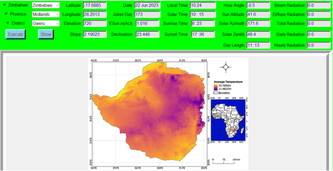
Figure 5. This interface offers capabilities of displaying and execution of command. Buttons were designed to execute command such as to run the algorithm for solar radiation estimation. Another capability of this interface is to display results from the algorithm. For a single randomly selected point within the study region the interface can display information that is recorded or executed by the algorithm. This information includes the geographical location (latitude, longitude, elevation in meters), terrain derivative (slope in degrees), time (local time, solar time, sunrise time, sunset time, day length). Solar geometry angles are also displayed, these includes solar zenith angle, hour angle, sun altitude, solar azimuth. Some of the outputs are displayed on the interface but the majority of the data are created and stored in a file folder system and can be retrieved and used in other GIS software’s. These datasets include raster files of Hourly radiation, Daily radiation and Monthly average radiation.
Figure 5. A snapshot of the BlueSky Interface.
3.2. Estimated Hourly Radiation
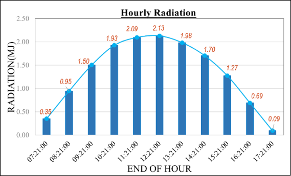
The BlueSky system is capable of calculating received hourly radiation for each day.
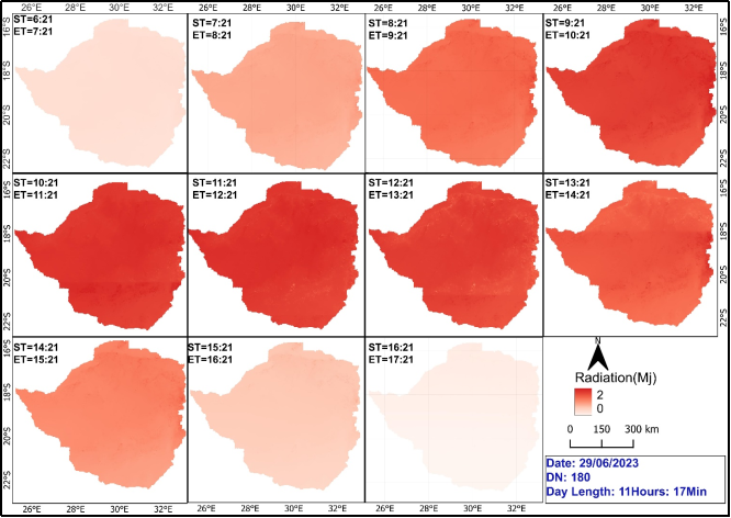
Figure 6 and 7 show how radiation varies on hourly intervals. The system managed to determine the temporal evolution in ground solar radiation from sunrise to sunset. The system starts calculating radiation immediately after sunrise. For example, on the 29
th of June 2023, sunrise was at 06:21am. Morning hours from 6:21am to 8:21am were dominated by radiation values of less than 0.9Mj as shown in
Figure 6. During morning hours sun angles were low and sun rays were hitting the surface at a tilted angle leading to much attenuation. On a clear day as time approaches midday from about 9:21am to 12:21am, large amounts of radiation of about 1.5Mj to 2.13Mj were received as depicted by
Figure 6. At these hours, the surface receives direct solar rays which signifies larger radiation amounts. During midday radiation intensities were large and the surface receives solar radiation around 2Mj. From about 11:21am, the surface received radiation of 2.09Mj with a peak of 2.13Mj at 12:21pm and 1.98Mj at 13:21pm. For Post midday from 14:21pm, there was a downward trend in received ground radiation from 1.7Mj to 0.09Mj at 17:21pm. Solar zenith angles increases as time moves away from midday; this signifies more attenuation as solar radiation travels much more distance in the atmosphere. Increase in radiation attenuation simply means decrease in ground received solar radiation. Hourly radiation shows a belly shaped curve when plotted against time as depicted in
Figure 6.
Figure 6. Hourly radiation graph.
Figure 7. Variation in hourly radiation map.
3.3. Estimated Daily Radiation
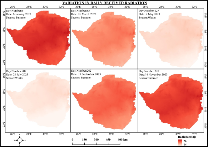
The total amount of radiation received on daily bases differs with day number as shown in
Figure 9. On clear days, radiation received for adjacent days tend to have less variance as shown by
Figure 8. On the contrary for day numbers that were further apart and day numbers in different seasons receive significantly different amounts of solar radiation as shown by
Figure 9. For example, on the 6
th January 2023 average radiation received was 24Mj, while on the 26
th July 2023, an average surface radiation received was 15Mj. As shown in
Figure 9, significant changes in daily radiation are evidenced on different days. As the days approach winter season daily radiation of about 18.5Mj to 14Mj were received. Summer days e.g October days received quite higher radiation of about 20Mj to 26MJ. Daily radiation differs because of the daily changes in declination angle and change in the sun earth distance. Solar intensity is inversely related to sun earth distance
| [18] | J. A. Duffie and W. A. Beckman, Solar Engineering of Thermal Processes, 4th ed. Hoboken, New Jersey: John Wiley & Sons, Inc., 2013. |
[18]
. When the earth is on the aphelion (normally in July e.g 6
th July for 2023) solar rays travel long distance and the radiation intensity is low. As shown in
Figure 9, radiation received on the 27
th July 2023 was less than 18Mj for most parts of the country. For that day and its adjacent days, the surface radiation was however lower than 18.5Mj. When the earth is on the perihelion (closer to the sun e.g 4
th January 2023), solar rays travel shorter distances and the radiation intensity was slightly higher than 24Mj.
| [29] | O. O. Apeh, O. K. Overen, and E. L. Meyer, ‘Monthly, Seasonal and Yearly Assessments of Global Solar Radiation, Clearness Index and Diffuse Fractions in Alice, South Africa’, Sustainability, vol. 13, no. 4, p. 2135, Feb. 2021, https://doi.org/10.3390/su13042135 |
[29]
found that when the earth is closer to or at the perihelion high ground solar radiation is received. As depicted in
Figure 9, for example on the 6
th January 2023, radiation above 24Mj was received.
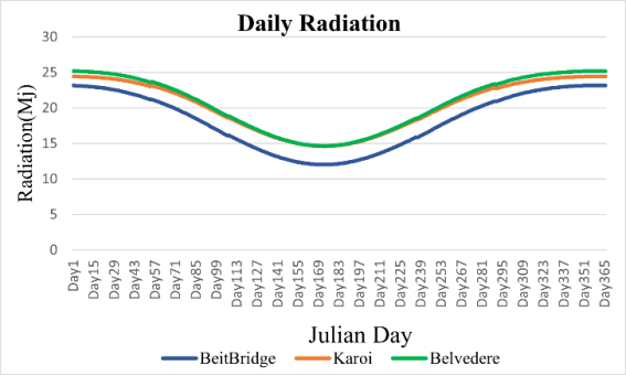
Figure 8 shows that two sites Belvedere and Beitbridge receives different amounts of radiation on daily basis. Belvedere receives a maximum of 25Mj in summers season and a minimum of 15Mj in winter season whilst Beitbridge receives a maximum of 23Mj in summer season and a minimum of 13Mj in winter season. This also shows that daily radiation varies with location as well.
Figure 8. Variation in Daily Radiation over 3 locations.
Figure 9. Daily Radiation Map.
3.4. Estimated Monthly Radiation
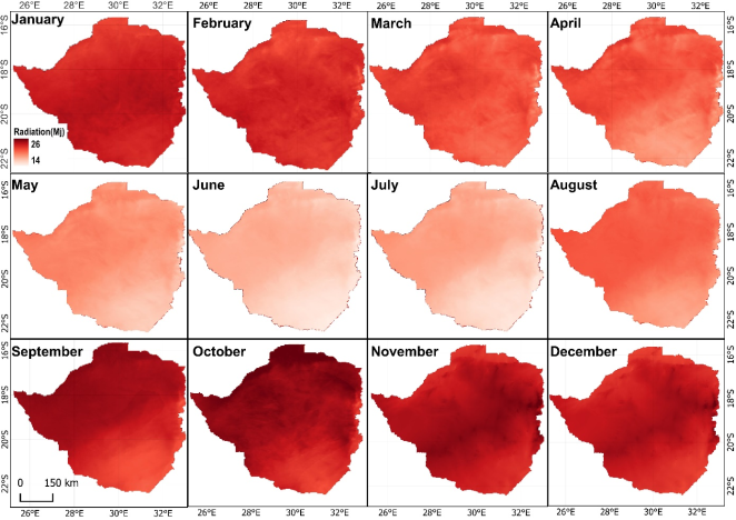
Monthly radiation maps were created and the results shown in
Figure 10. Radiation varies on monthly bases following changes in the declination angle and the sun earth distance. It is evidenced from
Figure 10 that in Zimbabwe, spring and summer seasons (that is the months of September to March), receives radiation of about 20Mj to 26Mj with the month of October having the highest surface solar radiation of 26Mj. As the earth moves closer to the sun and as the tilt angle between the sun and the centre of the earth approaches zero, radiation received tends to approach higher values. As the earth moves further away from the sun the radiation received tends to be less than 18.5Mj. This is because solar intensity is inversely proportional to sun earth distance
| [18] | J. A. Duffie and W. A. Beckman, Solar Engineering of Thermal Processes, 4th ed. Hoboken, New Jersey: John Wiley & Sons, Inc., 2013. |
[18]
. In summer season the sun is directly overhead the earth’s surface and the photons/ solar rays travels through a thinner atmosphere resulting in minimal attenuation and more received ground radiation
| [29] | O. O. Apeh, O. K. Overen, and E. L. Meyer, ‘Monthly, Seasonal and Yearly Assessments of Global Solar Radiation, Clearness Index and Diffuse Fractions in Alice, South Africa’, Sustainability, vol. 13, no. 4, p. 2135, Feb. 2021, https://doi.org/10.3390/su13042135 |
[29]
.
| [21] | C. Iradukunda and K. Chiteka, ‘Angstrom-Prescott Type Models for Predicting Solar Irradiation for Different Locations in Zimbabwe’, sv-jme, vol. 69, no. 1-2, pp. 32-48, Feb. 2023, https://doi.org/10.5545/sv-jme.2022.331 |
[21]
found out from their study that in Zimbabwe, radiation received are low for winter months (June, July and August) and high in summer months (October, November, December and January).
Figure 10 showed that the month of June receives low solar radiation of about 14Mj to 17Mj. This is because the earth is closer to the aphelion. When the earth is at the aphelion, solar rays travel a longer distance to the earth’s surface therefore radiation intensity is expected to be low. In winter the earth surface is tilted in relation to the sun therefore solar rays travels through thicker atmosphere leading to more attenuation and low received solar radiation
| [29] | O. O. Apeh, O. K. Overen, and E. L. Meyer, ‘Monthly, Seasonal and Yearly Assessments of Global Solar Radiation, Clearness Index and Diffuse Fractions in Alice, South Africa’, Sustainability, vol. 13, no. 4, p. 2135, Feb. 2021, https://doi.org/10.3390/su13042135 |
[29]
. In Zimbabwe the months of May, June and July are the peak of winter season evidenced by colder temperatures and less radiation intensities of about 14Mj to 18.5Mj. This was also evident in
Figure 11 where winter months have radiation values of less than 18.5Mj.
Figure 10. Monthly average radiation from January to December.
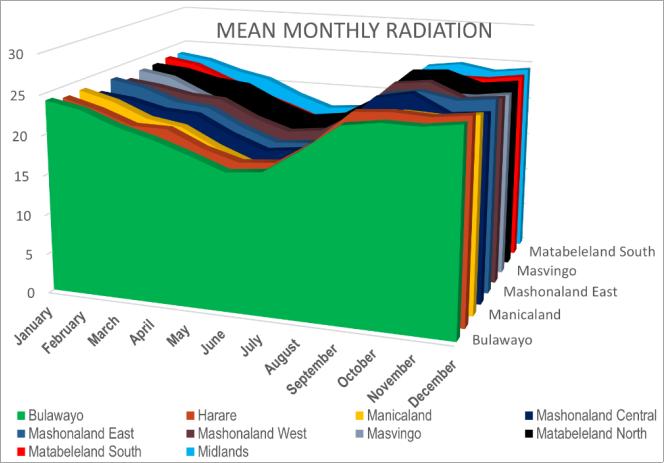
3.5. Estimated Monthly Radiation in Zimbabwe Provinces for Solar Energy
Figure 11 shows the monthly average received radiation for the 10 provinces of Zimbabwe. Seasonality variation in radiation is observed for all the provinces of Zimbabwe. At the beginning of the year radiation values were slightly higher above 23Mj and the trend declines towards June to about 14Mj. For all the 10 provinces, the average monthly radiation was less than 18Mj for the months of May, June and July. However, the month of August act as the transition month as it had moderate radiation of about 18Mj to 19.5Mj. The monthly radiation graph was rejuvenated from the month of August, and radiation values approached 26Mj in October and November. The months of September, October, November and December were evidenced by high radiation values above 24Mj. This result followed the same trend with the findings of
| [21] | C. Iradukunda and K. Chiteka, ‘Angstrom-Prescott Type Models for Predicting Solar Irradiation for Different Locations in Zimbabwe’, sv-jme, vol. 69, no. 1-2, pp. 32-48, Feb. 2023, https://doi.org/10.5545/sv-jme.2022.331 |
[21]
whom in their research observed that in Zimbabwe, monthly radiation forms a U-Shaped plot with the lowest values observed in May, June and July whilst highest values observed in October, September, December and January. For solar harvesting in order to curb solar energy problems in the nation, summer months provides a remedy. At the same time these months were the dry season of the nation and are associated with low river discharge and reduced water levels in Kariba dam
| [6] | R. Runganga and S. Mishi, ‘Modelling Electric Power Consumption, Energy Consumption and Economic Growth in Zimbabwe: Cointegration and Causality Analysis’, American Journal of Economics, 2020. |
[6]
thereby crippling hydroelectricity generation. However, for the same season when hydroelectric power generation is disadvantaged solar energy is widely available for all parts of the nation. For the months of September to February the nation can fully utilize the large quantities of solar energy.
Figure 11. Variation in Mean Monthly Radiation per province.
3.6. Statistical Evaluation of Monthly Radiation
The statistical analysis evaluated the performance of the developed system in estimating ground solar radiation. Mean monthly radiation insitu data were used to validate the mean monthly radiation data from the developed “
BlueSky” system. Pearson correlation R statistics was conducted to test the strength and direction of relationship between monthly insitu data and data from each model. The monthly correlation values for each dataset are as presented in
Table 3. A moderate association was observed for the month of Novemeber with R=0.48, whilst the rest of the months have a strong association (R=0.56). Winter months which are May and July exhibited very high association between BlueSky results and Insitu data, this implies the reliability of the developed system as its results were singing from the same hymn book with the reference data. To measure how well the modeled radiation data predicts ground received solar radiation, coefficient of determination was performed. A good model fit was observed for half of the year with an R
2 above 50%. The month of May stood taller with 79% significance between insitu and BlueSky. Although Pearson correlation R and coefficient of determination R
2 demonstrate a good relationship between insitu and predicted radiation dataset, these two statistical metrics are not enough, since models might underestimate or overestimate the amount of received solar radiation but still have high correlation, therefore other metrics were employed. RMSE was performed and average magnitude of difference between predicted and actual dataset was observed to be less than 2.9 for all the months were computed. The lowest discrepancy was observed on the month of October with a RMSE of 0.79. Normalized Mean Absolute Error (NMAE) was then used to calculate the absolute difference between in-situ and each modeled radiation data and to determine the average magnitude absolute error. All values closer to zero indicated better accuracy of the model as exhibited by the Months of February, September and October. From this research it was observed that data may have higher correlation at the same time containing larger residuals between predicted and observed. However computed statistical metrics proved that the Bluesky performs better in modelling clear sky ground solar radiation. Since the metrics provided compelling evidence in support of the developed systems, therefore results of the system can be used for decision marking in solar energy harnessing.
Table 3. Statistical Metrics.
Month | R | R | RMSE | NMAE |
January | 0.59 | 0.35 | 2.54 | 1.17 |
February | 0.74 | 0.54 | 1.18 | 0.89 |
March | 0.63 | 0.40 | 1.48 | 1.00 |
April | 0.79 | 0.62 | 2.77 | 1.36 |
May | 0.89 | 0.79 | 2.70 | 1.61 |
June | 0.66 | 0.44 | 2.67 | 1.47 |
July | 0.80 | 0.64 | 2.68 | 1.49 |
August | 0.78 | 0.61 | 2.67 | 1.55 |
September | 0.75 | 0.56 | 1.13 | 0.96 |
October | 0.57 | 0.32 | 0.79 | 0.76 |
November | 0.48 | 0.23 | 2.33 | 1.27 |
December | 0.61 | 0.38 | 2.89 | 1.32 |
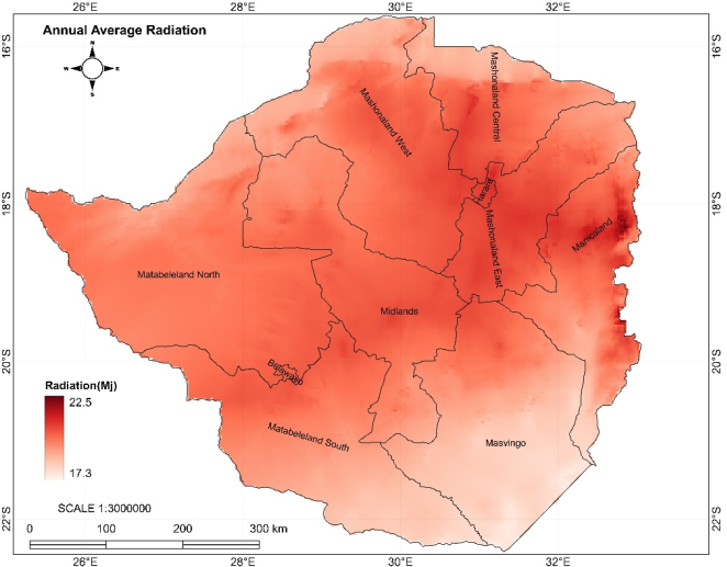
3.7. Estimated Mean Annual Radiation
From
Figure 12 it can be shown that annually the whole of Zimbabwe receives an average radiation which ranges between 17.3Mj to 22.5Mj. However, the average radiation varies per province with most northern, central and western parts falling within the high radiation belt. There is an upward gradient in radiation towards the western end of the Zimbabwe
| [30] | T. Hove and J. Gottsche, ‘Mapping global, diuse and beam solar radiation over Zimbabwe’, Renewable Energy, Oct. 1999. |
[30]
. Radiation amount declines towards the southern parts of the nation. This was evident in
Table 4 which shows there was a strong association between latitude and annual average radiation. Zimbabwe falls within the southern hemisphere and its latitude decreases towards the south. Decrease in latitude values strongly influence the amount of received radiation leading to decrease in radiation. Therefore, received radiation is partially proportional to latitude. However, some areas within the northern parts of Zimbabwe which have high latitude values tend to receive slightly less radiation compared to the general areas of the northern region. This was further clarified in
Table 5 which shows strong association between annual average radiation and elevation. The northern regions as well as the southern regions of Zimbabwe are dominated by low elevation values as shown by
Figure 2(a). Although the northern regions are within high latitude zone, some of these regions receive moderate annual radiation around 20Mj. These regions include the far northern parts of Mashonaland west, Mashonaland central, and Mashonaland east provinces. They all had moderate radiation values because their values were pulled down by their low elevation values as shown in
Figure 12. Above all the nation has abundant solar radiation which can be harnessed for energy use. Areas that receive larger amounts of solar radiation tend to output higher electricity energy. There is no consensus among researcher on the minimum amount of radiation for solar harvesting. However,
| [31] | U. Munkhbat and Y. Choi, ‘GIS-Based Site Suitability Analysis for Solar Power Systems in Mongolia’, Applied Sciences, vol. 11, no. 9, p. 3748, Apr. 2021, https://doi.org/10.3390/app11093748 |
[31]
stated that an amount of 14.4Mj is ideal for economic use of photovoltaic solar.
| [32] | K. Kamati, J. Smit, and S. Hull, ‘Multicriteria Decision Method for Siting Wind and Solar Power Plants in Central North Namibia’, Geomatics, vol. 3, no. 1, pp. 47-68, Dec. 2022, https://doi.org/10.3390/geomatics3010002 |
[32]
Also pointed out that 12.82Mj is required for cost effective solar operation. Judging from this assertion, Zimbabwe provinces exceeded the two proposed thresholds, thus solar radiation can be abundantly harvested to solve the prevailing energy problem in the nation. Nevertheless, there are other factors that draws back the amount of energy to be harnessed, and the reason for site suitability analysis conducted in this study.
Table 4. Elevation and Radiation relationship.
Correlations |
| Elevation | Radiation |
Elevation | Pearson Correlation | 1 | .617** |
Sig. (2-tailed) | | <.001 |
N | 500 | 500 |
Radiation | Pearson Correlation | .617** | 1 |
Sig. (2-tailed) | <.001 | |
N | 500 | 500 |
** Correlation is significant at the 0.01 level (2-tailed). |
Table 5. Latitude and Radiation relationship.
Correlations |
| Latitude | Radiation |
Latitude | Pearson Correlation | 1 | .545** |
Sig. (2-tailed) | | <.001 |
N | 500 | 500 |
Radiation | Pearson Correlation | .545** | 1 |
Sig. (2-tailed) | <.001 | |
N | 500 | 500 |
** Correlation is significant at the 0.01 level (2-tailed). |
Figure 12. Annual average radiation.
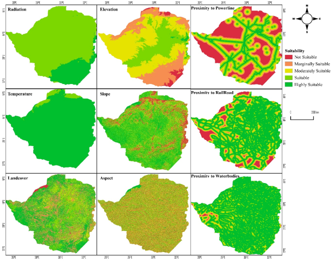
3.8. Site Suitability Factors
Table 6 shows how each site suitability factors were classified into suitability classes. In the southern hemisphere, north facing slopes are more suitable followed by North East and North West facing slopes. Gentle areas where slope is less than 3 are more preferable for solar farming as they receive direct solar rays. Steep slopes are the less preferable since they often cast shadows to solar panels
| [28] | I. I. Opeyemi, A. S. Abayomi, and G. Suara, ‘Site Suitability Assessment for Solar Photovoltaic Power Plant in FCT-Abuja, Nigeria: A Geographic Information System (GIS) and Analytical Hierarchy Process (AHP) Approach’, 2022. |
[28]
.
Table 4 showed that there is a strong correlation between elevation and radiation therefore, high elevation areas are most suitable for solar farming. Areas with high elevations receives high solar radiation and tend to produce more electricity
| [28] | I. I. Opeyemi, A. S. Abayomi, and G. Suara, ‘Site Suitability Assessment for Solar Photovoltaic Power Plant in FCT-Abuja, Nigeria: A Geographic Information System (GIS) and Analytical Hierarchy Process (AHP) Approach’, 2022. |
[28]
. It is of economic advantage to construct solar panels closer to roads, powerlines, and water bodies. The closer the site is to railroad network reduces the cost of transporting raw materials and workers. The closer the site is to existing transmission lines reduces the cost of linking the solar power plant to the electricity grid
| [5] | S. Ziuku, L. Seyitini, B. Mapurisa, D. Chikodzi, and K. Van Kuijk, ‘Potential of Concentrated Solar Power (CSP) in Zimbabwe’, Energy for Sustainable Development, vol. 23, pp. 220-227, Dec. 2014, https://doi.org/10.1016/j.esd.2014.07.006 |
[5]
and those sites within 5km are most suitable. Water is required for cleaning and cooling solar panels therefore sites closer to water bodies are most suitable as shown by
Table 6. In terms of landcover, bare areas are most suitable for siting solar panels since there is little harm on the forest ecosystem, followed by shrubland and the least is water. Increase in temperature tend to retard PV output. As surface temperature increases, solar module temperature increases as well which leads to an exponential increase in current output leading to linear decline in voltage
| [32] | K. Kamati, J. Smit, and S. Hull, ‘Multicriteria Decision Method for Siting Wind and Solar Power Plants in Central North Namibia’, Geomatics, vol. 3, no. 1, pp. 47-68, Dec. 2022, https://doi.org/10.3390/geomatics3010002 |
[32]
. As temperature exceeds 25°C voltage outputs starts to drop. Areas with temperature below 25°C are more suitable. Since there is no consensus among researchers on the minimum accepted radiation for solar farming, however this research adopts
| [31] | U. Munkhbat and Y. Choi, ‘GIS-Based Site Suitability Analysis for Solar Power Systems in Mongolia’, Applied Sciences, vol. 11, no. 9, p. 3748, Apr. 2021, https://doi.org/10.3390/app11093748 |
[31]
proposed 14.4 Mj as suitable for large scale solar farming. The suitability of each factor is shown in
Table 6 and
Figure 13. These suitability factors were used to determine the overall land suitability for solar harvesting.
Table 6. Land suitability factors.
Factor | Map | Classification | Classified Map | AHP Weight |
Radiation (Mj) | 
| <19 | 4 | 
| 17% |
≥ 19 | 5 |
Temperature (°C) | 
| <25 | 5 | 
| 13% |
≥25 | 4 |
Landcover | 
| Forest & Water | 1 | 
| 13% |
Built Up | 2 |
Crop land | 3 |
Shrub land | 4 |
Bare land | 5 |
Elevation (m) | 
| <450 | 1 | 
| 12% |
450-900 | 2 |
900-1350 | 3 |
1350-1800 | 4 |
>1800 | 5 |
Slope (%) | 
| <3 | 5 | 
| 15% |
3-5 | 4 |
5-8 | 3 |
8-11 | 2 |
>11 | 1 |
Aspect | 
| North | 5 | 
| 11% |
NE & NW | 4 |
E & W | 3 |
SE & SW | 2 |
S | 1 |
Proximity to Poweline (km) | 
| <5 | 5 | 
| 5% |
5-10 | 4 |
10-15 | 3 |
15-20 | 2 |
>20 | 1 |
Proximity to RailRoad (km) | 
| <5 | 5 | 
| 6% |
5-10 | 4 |
10-15 | 3 |
15-20 | 2 |
>20 | 1 |
Proximity to River (km) | 
| <5 | 5 | 
| 5% |
5-10 | 4 |
10-15 | 3 |
15-20 | 2 |
>20 | 1 |
Figure 13. Suitability Factors.
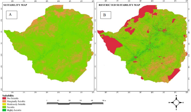
3.9. Site Suitability for Solar Mapping in Zimbabwe
Weighted overlay analysis was used to determine the suitability of each site using factors mentioned in
Figure 13 and
Table 6. It is evidenced from
Figure 14(a) that Zimbabwe is dominated by suitable areas for solar farming followed by moderately suitable sites. The suitability of a site is a combination of different weighted factors. Since most areas were deemed highly suitable by already identified factors, most areas were classified as moderately suitable. Although most areas are highly suitable, not every suitable site can be used for development due to local laws and regulations. Areas such as national parks, safaris, protected areas and airports are restricted for development. As shown by the restricted suitability map in
Figure 14(b) most areas are not suitable because of the locally imposed restrictions. All areas within 100m from railroad are considered restricted because locating solar plant close to road is a challenge in terms of security, road expansion, even accidents
| [33] | A. Alhammad, Q. (Chayn) Sun, and Y. Tao, ‘Optimal Solar Plant Site Identification Using GIS and Remote Sensing: Framework and Case Study’, Energies, vol. 15, no. 1, p. 312, Jan. 2022, https://doi.org/10.3390/en15010312 |
[33]
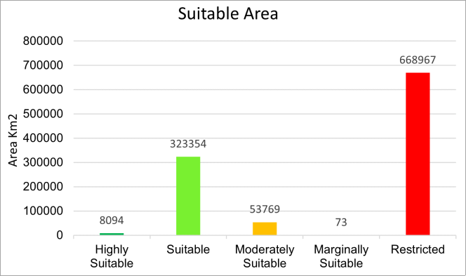
. Powerlines have a servitude which demarcates areas to be excluded for and these areas are restricted as well. All areas very close to water reservoirs such as rivers, and dams are restricted by local laws, also to avoid flooding of solar farms. Restricted areas occupy most parts of the country, followed by suitable areas, moderately suitable, highly suitable and marginally suitable in that order as shown by
Figure 15. From the conducted site suitability analysis 0.77% was highly suitable, 30.65% was suitable, 5.1% was moderately suitable and 63.42% fell under restricted areas.
Figure 14. Solar Suitability Map for Zimbabwe.
Figure 15. Suitability Area.
From
Figure 15, highly suitable areas occupy 8,094
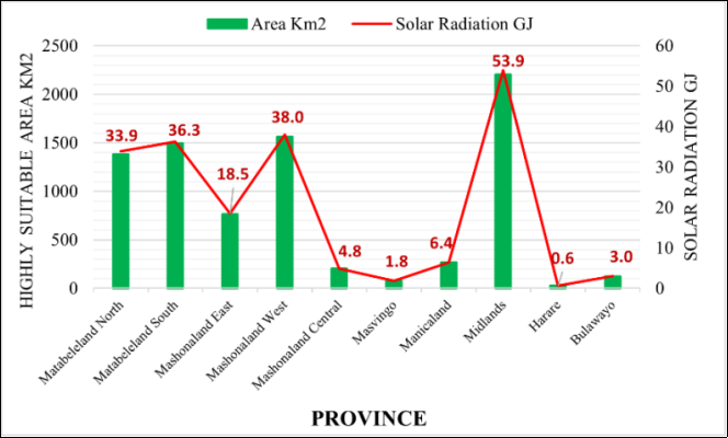
km2. Highly suitable areas have gentle slope, high elevation, bare areas, closer to water, closer to railroad, close to powerline, north, northwest, North West facing slopes, high radiation, temperature less than 25°C. Midlands province has largest highly suitable area, followed by Mashonaland West, Matabeleland South and Matabeleland North. It can be observed that, every province in Zimbabwe have the potential to produce desirable amounts of solar energy.
Table 7 shows the area that is highly suitable for solar harvesting, total radiation received in that area and the potential efficient energy be harvested per province.
| [34] | G. Najafi, B. Ghobadian, R. Mamat, T. Yusaf, and W. H. Azmi, ‘Solar energy in Iran: Current state and outlook’, Renewable and Sustainable Energy Reviews, vol. 49, pp. 931-942, Sep. 2015, https://doi.org/10.1016/j.rser.2015.04.056 |
[34]
Considered only 1% of the suitable area with a 10% solar system efficiency to harness solar energy and found out that in a day 9 million megawatts (MW) of energy can be obtained. In this study, by considering an area of 80.94 km
2 which is 1% of the total highly suitable area whilst using a solar system with 10% efficiency, 197.41GJ can be harvested in Zimbabwe as presented in
Table 7 and
Figure 16. With good storage system this energy is more than enough to curb Zimbabwe’s prevailing energy crisis.
Figure 16. Highly Suitable Area and Total Radiation.
Table 7. Provincial Total radiation received on highly suitable area.
Province | Surface Area Km2 | Highly Suitable Area Km2 | Percentage of High Suitable Area | Total Received Radiation GJ | Potential efficient energy GJ |
Matabeleland North | 76065.62 | 1380.83 | 1.82% | 33937.21 | 3393.72 |
Matabeleland South | 54325.81 | 1492.66 | 2.75% | 36296.48 | 3629.65 |
Mashonaland East | 32163.68 | 761.62 | 2.37% | 18498.86 | 1849.89 |
Mashonaland West | 28200.96 | 1560.20 | 5.53% | 38036.84 | 3803.68 |
Mashonaland Central | 57812.57 | 201.89 | 0.35% | 4839.74 | 483.97 |
Masvingo | 56462.41 | 77.57 | 0.14% | 1844.44 | 184.44 |
Manicaland | 35820.77 | 266.99 | 0.75% | 6390.21 | 639.0 |
Midlands | 49500.13 | 2203.27 | 4.45% | 53906.58 | 5390.66 |
Harare | 940.21 | 26.27 | 2.79% | 639.65 | 63.97 |
Bulawayo | 548.26 | 122.58 | 22.36% | 3017.43 | 301.74 |